Welcome to the Principal Component Analysis (PCA) post. I hope you have gone through all the previous posts on Machine Learning, Supervised Learning and Unsupervised Learning.
Principal Component Analysis is an unsupervised learning algorithm that is used for the dimensionality reduction in machine learning.
PCA is a dimensionality-reduction method that is often used to reduce the dimensionality of large data sets, by transforming a large set of variables into a smaller one that still contains most of the information in the large set.
Reducing the number of variables of a data set naturally comes at the expense of accuracy, but the trick in dimensionality reduction is to trade a little accuracy for simplicity.
The reason behind reducing the features in a large data set is because smaller data sets are easier and faster to analyze, explore and visualize for machine learning algorithms without large variables to process which consumes a lot of time and computational power.
So to sum up, the idea of PCA is simple — reduce the number of variables of a data set, while preserving as much information as possible.
Step wise Explanation of PCA:
Step 1 – Standardization
The aim of this step is to standardize the range of the continuous initial variables so that each one of them contributes equally to the analysis. More specifically, the reason why it is critical to perform standardization prior to PCA, is that the latter is quite sensitive regarding the variances of the initial variables.
Feature Scaling is a technique to standardize the independent features present in the data in a fixed range. If feature scaling is not done, then a machine learning algorithm tends to weigh greater values, higher and consider smaller values as the lower values, regardless of the unit of the values.
Example: If an algorithm is not using the feature scaling method then it can consider the value 3000 meters to be greater than 5 km but that’s actually not true and in this case, the algorithm will give wrong predictions. So, we use Feature Scaling to bring all values to the same magnitudes and thus, tackle this issue.
Mathematically, this can be done by subtracting the mean and dividing by the standard deviation for each value of each variable.
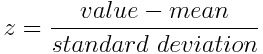
Once the standardization is done, all the variables will be transformed to the same scale.
Step 2: Covariance Matrix Computation
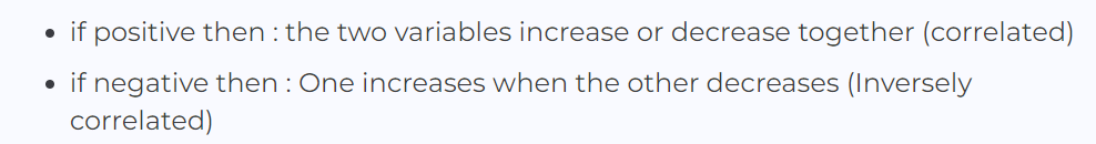
The aim of this step is to understand how the variables of the input data set are varying from the mean with respect to each other, or in other words, to see if there is any relationship between them.
It’s actually the sign of the covariance that matters :
Step 3 – Identify Principal Components
Principal components are new variables that are constructed as mixtures of the initial variables. These combinations are done in such a way that the new variables (i.e., principal components) are uncorrelated and most of the information within the initial variables is compressed into the first components.
So, the idea is 10-dimensional data gives you 10 principal components, but PCA tries to put maximum possible information in the first component, then maximum remaining information in the second and so on.
Scree plot – Displays how much variance each PCA captures from the data. In the below figure it shows that the principal component 1 captures almost 40 % of the total information from the data set. PC 1 explains 40% of the variance from the data.
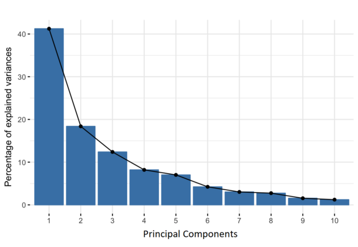
We have to choose a particular number of Principal Component so that we get the significant percentage of variance with less amount of principal components.
A widely applied approach is to decide on the number of principal components by examining a scree plot. By eyeballing the scree plot above, and looking for a point at which the proportion of variance explained by each subsequent principal component drops off. This is often referred to as an elbow in the scree plot. An ideal curve should be steep, then bends at an “elbow” — this is your cutting-off point — and after that flattens out.
Based on that we could select the Principal Component as 4 in the above figure. Lets calculate the approx variance now captured in the first 4 components.
PC 1 – 41, PC 2 – 18, PC 3 – 13 and PC 4 – 8. Therefore, a total of 4 Principal components explains 80% of the variance from the total data.
Step 4 – Feature Vector
In this step, what we do is, to choose whether to keep all these components or discard those of lesser significance (of low eigenvalues) and form with the remaining ones a matrix of vectors that we call Feature vector.
Use this transformed data in the whichever model you want to use. Now the model’s accuracy will be higher as we have removed the unnecessary features from the data.
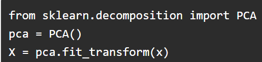
Python code for PCA:
In layman’s terms, Principal Component Analysis (PCA) falls under the category of unsupervised machine learning algorithms where the model learns without any target variable. PCA has been specifically used in the area of Dimensionality Reduction to avoid the curse of dimension.
For example – PCA reduces the 100 features in a dataset (just for example) into some specified number of M features where m can be specified explicitly.
- Input = Feature1 | Feature2 | Feature3 | Feature4 | Feature5 | Feature6 … Feature100
- Imagine you are trying to get 3 principal components (M = 3)
- Output = PCA1 | PCA2 | PCA3
Now the dimensionality is reduced from 100 features to 3 Principal components in which all the 3 principal components gives the meaning of 100 features.
PCA is not an algorithm where you can get a solution formula or something like regression analysis. It is just a way to cut down the dimension.
Thanks for reading. Do read the further posts. Please feel free to connect with me if you have any doubts. Do follow, support, like and subscribe this blog.
