Welcome to the Part 2 of Machine Learning. If you haven’t gone through the Part 1 of ML click here Part-1. In this post we are going to discuss about the core statistics which helps in understanding ML.
Machine Learning is nothing but the combination of statistics with other fields. So in order to clearly understand Machine Learning you need to know some of the core statistics which is very important. Some of them are Standard Deviation, Correlation, Bayes Theorem, Feature Selection and Feature Extraction.
Standard Deviation
Standard deviation is a measure of the amount of variation or dispersion of a set of values. It measures the Spread of a group of numbers from the mean. Standard Deviation is denoted using σ.
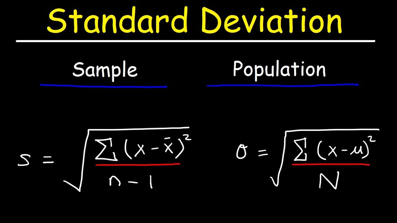
where,
N – size of population & n – size of sample μ – population mean & x̅ – sample mean x – each value of the data given
Example – 1) 15,15,15,14,16 2) 2,7,14,22,30
From the above given example, we find that the mean value of both 1) and 2) are same. But the values in 2) are clearly spread out. Therefore 2) has high Standard deviation compared to the 1). So, if a set has low Standard deviation, then the values are not spread too much or in other words most of the values are closer to the mean.
Correlation
A machine learning algorithm often involves some type of correlation among the data. Correlation refers to the linear relationship between two variables. It ranges from -1 to +1. It expresses the strength of the relationship between 2 variables.
Types of correlation
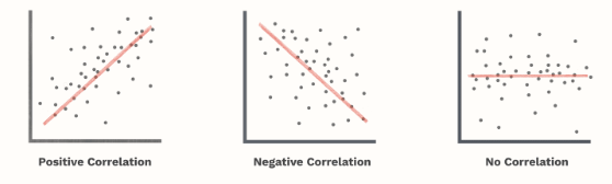
There are three types of correlation. They are
- Positive Correlation
- Negative Correlation
- No Correlation
Positive Correlation – When the value of one variable increases, then the value of other variable also increases. Ex – Suppose there is a 0.7 correlation between income and spending. If income increases by $100, then the value of spending will also increase by $70 ($100 X 0.7).
Negative Correlation – When the value of one variable increases, then the value of other variable decreases. It denoted an inverse relationship.
No Correlation – If the correlation is zero, then there is no relationship between the 2 variables.
Feature Selection
Feature Selection is the process in which we select only the features or variables which contributes more to our output. This is followed to reduce the irrelevant variables which usually decreases the accuracy of the model.
Feature Extraction
It is a process of Dimension Reduction in which the input data is reduced to few groups which can be managed. It aims to reduce the number of features in the data by creating new features from existing one and then discarding the original features. If there are so many variables in the dataset, we perform Feature extraction. It helps in boosting the accuracy of the model.
Example – Take a computer model which does image recognition and identifies whether the person is male or female. It is very easy to identify them in case of humans. But for a machine to identify we need to train it with data like shown in the below example.
The below table shows some features which a male face possess which differs male face from female face . From that you can get a basic understanding about how we train machines to predict the model.
Features Male
Eyebrows | Thicker and straighter
Face shape | Longer and larger, with more of a square shape
Jawbone | Square, wider, and sharper
Neck | Adam’s apple
Bayes’ Theorem
This theorem is a way of finding a probability when we know certain other probabilities. It describes the probability of an event, based on prior knowledge that might be related to that event.
Conditional probability – Measures the probability of an event occurring given that another event has already occurred.
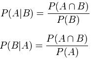
P(A|B) = Probability of A given B has occurred.
P (A ⋂ B) = P(B | A) * P(A)
Bayes Theorem = P (A | B) = ( P(B | A) * P(A) ) / P(B)
Example – 100 people gather at a function and you count how many wear pink or not, and if a man or not, and get these data,
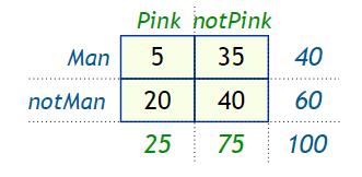
Now calculate some of the probabilities,
- The probability of wearing pink is P(Pink) = 25 / 100 = 0.25
- The probability of being a man is P(Man) = 40 / 100 = 0.4
- The probability that a man wears pink is P(Pink|Man) = 5 / 40 = 0.125
From these probabilities is it possible to find P( Man | Pink) ?
Yes we can find it using the Bayes’ Theorem formula. The probability that a person wearing pink is a man P (Man | Pink).
P(Man|Pink) = ( P(Man) * P(Pink | Man) ) / P(Pink)
P(Man|Pink) = (0.4 × 0.125) / 0.25 = 0.2
So, we found the probability using Bayes’ theorem.
Thanks for reading. Do read the further posts. Please feel free to connect with me if you have any doubts. Do follow, support, like and subscribe this blog.
Fact of the day:
51% of internet traffic is non-human. 31% is made up from hacking programs, spammers and malicious phishing.
