Techno Hunter

Spam Detection using Multinomial Naive Bayes

Welcome to the Spam Detection using Multinomial Naive Bayes post. I hope you have gone through all the previous posts on Machine Learning, Supervised Learning and Unsupervised Learning.

Spam Detection

Whenever you submit details about your email or contact number on any platform, it has become easy for those platforms to market their products by advertising them by sending emails or by sending messages directly to your contact number.

This results in lots of spam alerts and notifications in your inbox. This is where the task of spam detection comes in. Spam detection means detecting spam messages or emails by understanding text content so that you can only receive notifications about messages or emails that are very important to you.

If spam messages are found, they are automatically transferred to a spam folder and you are never notified of such alerts. This helps to improve the user experience, as many spam alerts can bother many users.

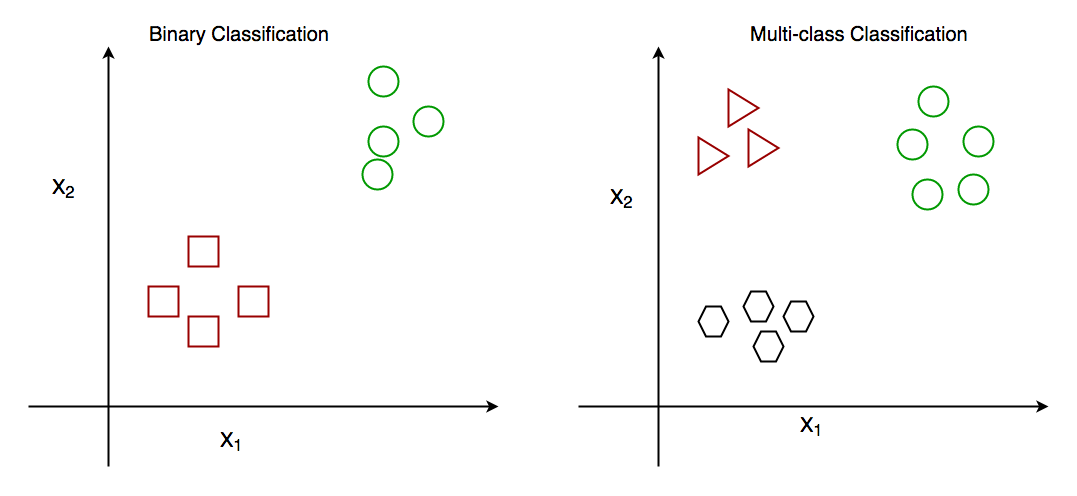
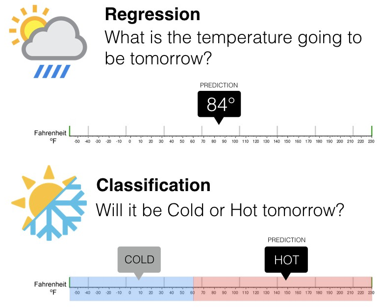
Classification problems can be broadly split into two categories: binary classification problems, and multi-class classification problems. Binary classification means there are only two possible label classes, e.g. a patient’s condition is cancerous or it isn’t, or a financial transaction is fraudulent or it is not.

Multi-class classification refers to cases where there are more than two label classes. An example of this is classifying the sentiment of a movie review into positive, negative, or neutral.

Gmail Spam Detection

We all know the data Google has, is not obviously in paper files. They have data centers which maintain the customers data. Before Google/Gmail decides to segregate the emails into spam or not spam category, before it arrives to your mailbox, hundreds of rules apply to those email in the data centers. These rules describe the properties of a spam email. There are common types of spam filters which are used by Gmail/Google —

Blatant Blocking- Deletes the emails even before it reaches to the inbox.

Bulk Email Filter- This filter helps in filtering the emails that are passed through other categories but are spam.

Category Filters- User can define their own rules which will enable the filtering of the messages according to the specific content or the email addresses etc.

Null Sender Disposition- Dispose of all messages without an SMTP envelope sender address. Remember when you get an email saying, “Not delivered to xyz address”.

Null Sender Header Tag Validation- Validate the messages by checking security digital signature.

There are ways to avoid spam filtering and send your emails straight to the inbox. To learn more about Gmail spam filter please watch this informational video from Google.

Detecting spam alerts in emails and messages is one of the main applications that every big tech company tries to improve for its customers. Apple’s official messaging app and Google’s Gmail are great examples of such applications where spam detection works well to protect users from spam alerts. So, if you are looking to build a spam detection system, this post is for you.

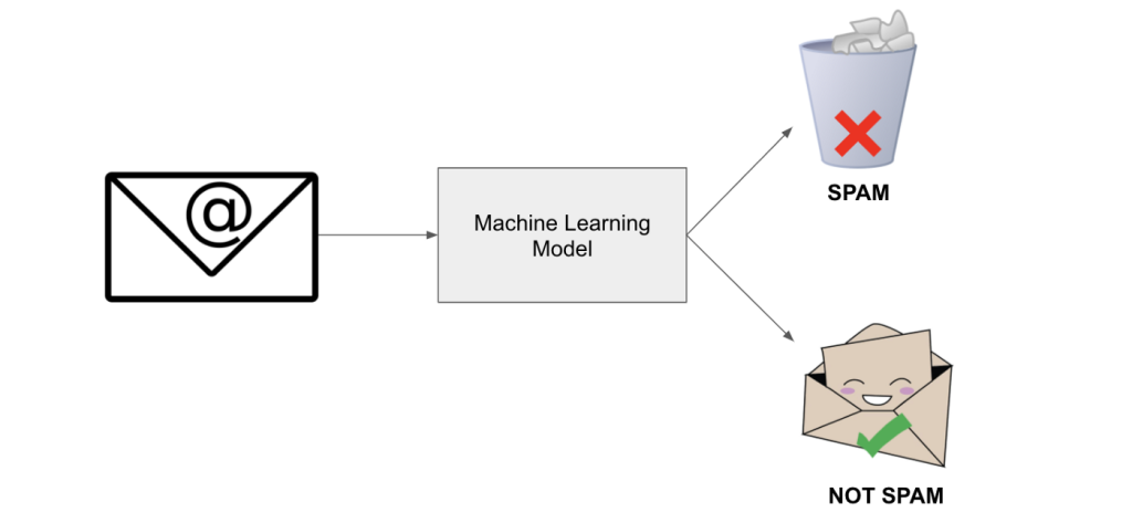
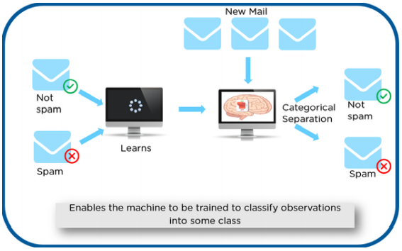
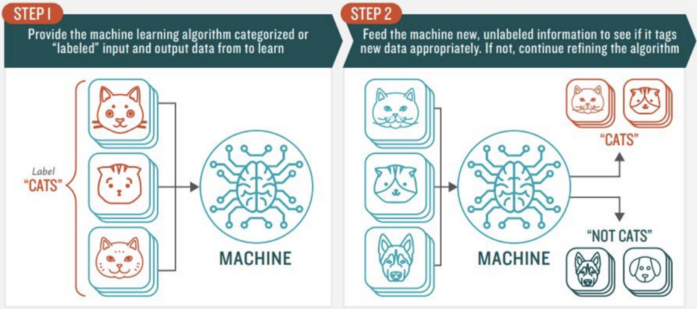
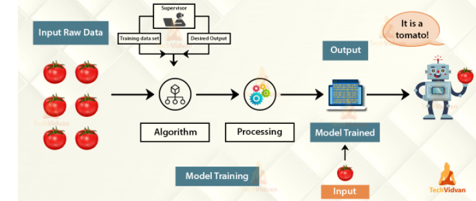
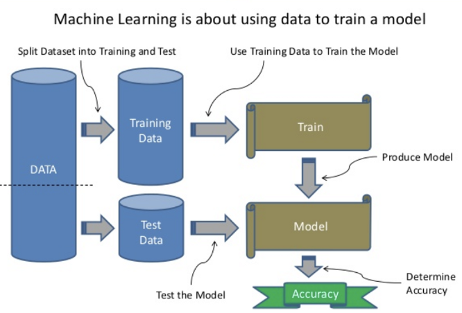
We are hoing to create a Spam Classifier system which distinguishes between Spam and Not Spam mails in the E-mail inbox. For that first we need a dataset which contains some examples of the mails which are spam and not spam. Then based on that data, we have to train the model. After the model is trained, then we have to test the model. After it is done and once we got high accuracy the model can be deployed.

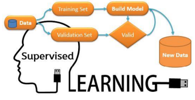
The above given Spam classifier is an example of Supervised Machine Learning. That is just a example of how it works.

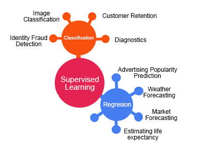
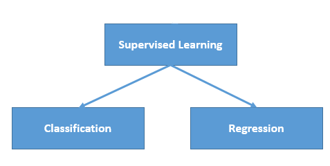
The Classification algorithm is a Supervised Learning technique that is used to identify the category of new observations on the basis of training data. In Classification, a program learns from the given dataset or observations and then classifies new observation into a number of classes or groups.

This application of Spam Detection comes under Classification. So, we are gonna use a Classification algorithm. There are many algorithms for Classification.

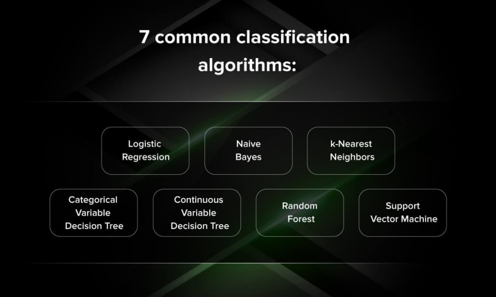
For this project, we are gonna use Naive Bayes Algorithm.

What is the Multinomial Naive Bayes?

Multinomial Naive Bayes algorithm is a probabilistic learning method that is mostly used in Natural Language Processing (NLP). The algorithm is based on the Bayes theorem and predicts the tag of a text such as a piece of email or newspaper article. It calculates the probability of each tag for a given sample and then gives the tag with the highest probability as output.

Naive Bayes classifier is a collection of many algorithms where all the algorithms share one common principle, and that is each feature being classified is not related to any other feature. The presence or absence of a feature does not affect the presence or absence of the other feature.

How Multinomial Naive Bayes works?

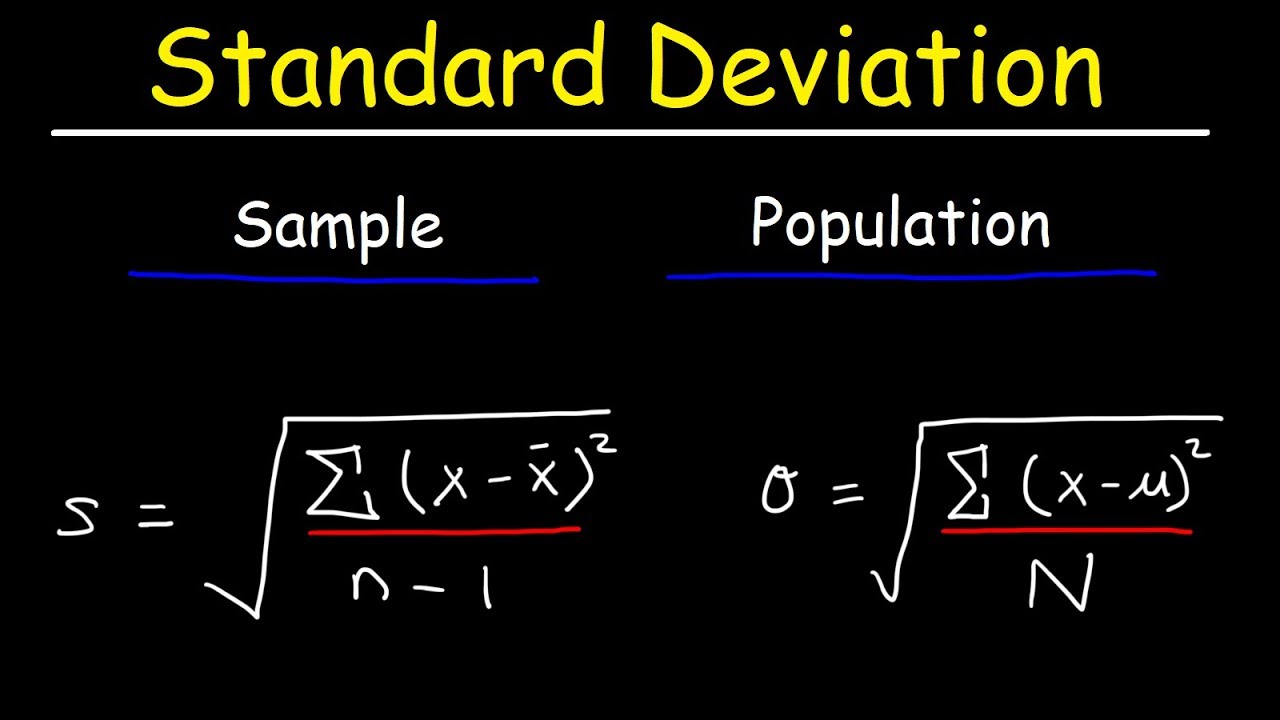
Naive Bayes is a powerful algorithm that is used for text data analysis and with problems with multiple classes. To understand Naive Bayes theorem’s working, it is important to understand the Bayes theorem concept first as it is based on the latter.

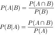
Bayes theorem, formulated by Thomas Bayes, calculates the probability of an event occurring based on the prior knowledge of conditions related to an event. It is based on the following formula:

P(A|B) = P(A) * P(B|A)/P(B)

Where we are calculating the probability of class A when predictor B is already provided.

P(B) = prior probability of B

P(A) = prior probability of class A

P(B|A) = occurrence of predictor B given class A probability

This formula helps in calculating the probability of the tags in the text.

Let us understand the Naive Bayes algorithm with an example. In the below given table, we have taken a data set of weather conditions that is sunny, overcast, and rainy. Now, we need to predict the probability of whether the players will play based on weather conditions.

Training Data Set

Weather

Sunny

Overcast

Rainy

Sunny

Overcast

Rainy

Sunny

Rainy

Sunny

Overcast

Rainy

Play

Yes

This can be easily calculated by following the below given steps:

Create a frequency table of the training data set given in the above problem statement. List the count of all the weather conditions against the respective weather condition.

Weather	Yes	No
Sunny	3	2
Overcast	4	0
Rainy	2	3
Total	9	5

Find the probabilities of each weather condition and create a likelihood table.

Weather	Yes	No
Sunny	3	2	=5/14(0.36)
Overcast	4	0	=4/14(0.29)
Rainy	2	3	=5/14(0.36)
Total	9	5
	=9/14 (0.64)	=5/14 (0.36)

Calculate the posterior probability for each weather condition using the Naive Bayes theorem. The weather condition with the highest probability will be the outcome of whether the players are going to play or not.

Use the following equation to calculate the posterior probability of all the weather conditions:

P(A|B) = P(A) * P(B|A)/P(B)

After replacing variables in the above formula, we get:

P(Yes|Sunny) = P(Yes) * P(Sunny|Yes) / P(Sunny)

Take the values from the above likelihood table and put it in the above formula.

P(Sunny|Yes) = 3/9 = 0.33, P(Yes) = 0.64 and P(Sunny) = 0.36

Hence, P(Yes|Sunny) = (0.64*0.33)/0.36 = 0.60

P(No|Sunny) = P(No) * P(Sunny|No) / P(Sunny)

Take the values from the above likelihood table and put it in the above formula.

P(Sunny|No) = 2/5 = 0.40, P(No) = 0.36 and P(Sunny) = 0.36

P(No|Sunny) = (0.36*0.40)/0.36 = 0.6 = 0.40

The probability of playing in sunny weather conditions is higher. Hence, the player will play if the weather is sunny.

Similarly, we can calculate the posterior probability of rainy and overcast conditions, and based on the highest probability; we can predict whether the player will play.

Hope you got an overall understanding about the project – Spam Detection using Multinomial Naive Bayes. This is just the theory part. I have also used Python programming language for this project, coded the project and created a Spam Classifier.

Do check the code in my Github profile and try it from your end. Github Link – https://github.com/muhil17/Spam-Detection-using-Multinomial-Naive-Bayes

Thanks for reading. Do read the further posts. Please feel free to connect with me if you have any doubts. Do follow, support, like and subscribe this blog.

Principal Component Analysis

Welcome to the Principal Component Analysis (PCA) post. I hope you have gone through all the previous posts on Machine Learning, Supervised Learning and Unsupervised Learning.

Principal Component Analysis is an unsupervised learning algorithm that is used for the dimensionality reduction in machine learning.

PCA is a dimensionality-reduction method that is often used to reduce the dimensionality of large data sets, by transforming a large set of variables into a smaller one that still contains most of the information in the large set.

Reducing the number of variables of a data set naturally comes at the expense of accuracy, but the trick in dimensionality reduction is to trade a little accuracy for simplicity.

The reason behind reducing the features in a large data set is because smaller data sets are easier and faster to analyze, explore and visualize for machine learning algorithms without large variables to process which consumes a lot of time and computational power.

So to sum up, the idea of PCA is simple — reduce the number of variables of a data set, while preserving as much information as possible.

Step wise Explanation of PCA:

Step 1 – Standardization

The aim of this step is to standardize the range of the continuous initial variables so that each one of them contributes equally to the analysis. More specifically, the reason why it is critical to perform standardization prior to PCA, is that the latter is quite sensitive regarding the variances of the initial variables.

Feature Scaling is a technique to standardize the independent features present in the data in a fixed range. If feature scaling is not done, then a machine learning algorithm tends to weigh greater values, higher and consider smaller values as the lower values, regardless of the unit of the values.

Example: If an algorithm is not using the feature scaling method then it can consider the value 3000 meters to be greater than 5 km but that’s actually not true and in this case, the algorithm will give wrong predictions. So, we use Feature Scaling to bring all values to the same magnitudes and thus, tackle this issue.

Mathematically, this can be done by subtracting the mean and dividing by the standard deviation for each value of each variable.

Principal Component Analysis Standardization

Once the standardization is done, all the variables will be transformed to the same scale.

Step 2: Covariance Matrix Computation

The aim of this step is to understand how the variables of the input data set are varying from the mean with respect to each other, or in other words, to see if there is any relationship between them.

It’s actually the sign of the covariance that matters :

Step 3 – Identify Principal Components

Principal components are new variables that are constructed as mixtures of the initial variables. These combinations are done in such a way that the new variables (i.e., principal components) are uncorrelated and most of the information within the initial variables is compressed into the first components.

So, the idea is 10-dimensional data gives you 10 principal components, but PCA tries to put maximum possible information in the first component, then maximum remaining information in the second and so on.

Scree plot – Displays how much variance each PCA captures from the data. In the below figure it shows that the principal component 1 captures almost 40 % of the total information from the data set. PC 1 explains 40% of the variance from the data.

We have to choose a particular number of Principal Component so that we get the significant percentage of variance with less amount of principal components.

A widely applied approach is to decide on the number of principal components by examining a scree plot. By eyeballing the scree plot above, and looking for a point at which the proportion of variance explained by each subsequent principal component drops off. This is often referred to as an elbow in the scree plot. An ideal curve should be steep, then bends at an “elbow” — this is your cutting-off point — and after that flattens out.

Based on that we could select the Principal Component as 4 in the above figure. Lets calculate the approx variance now captured in the first 4 components.

PC 1 – 41, PC 2 – 18, PC 3 – 13 and PC 4 – 8. Therefore, a total of 4 Principal components explains 80% of the variance from the total data.

Step 4 – Feature Vector

In this step, what we do is, to choose whether to keep all these components or discard those of lesser significance (of low eigenvalues) and form with the remaining ones a matrix of vectors that we call Feature vector.

Use this transformed data in the whichever model you want to use. Now the model’s accuracy will be higher as we have removed the unnecessary features from the data.

Python code for PCA:

In layman’s terms, Principal Component Analysis (PCA) falls under the category of unsupervised machine learning algorithms where the model learns without any target variable. PCA has been specifically used in the area of Dimensionality Reduction to avoid the curse of dimension.

For example – PCA reduces the 100 features in a dataset (just for example) into some specified number of M features where m can be specified explicitly.

Input = Feature1 | Feature2 | Feature3 | Feature4 | Feature5 | Feature6 … Feature100
- Imagine you are trying to get 3 principal components (M = 3)
Output = PCA1 | PCA2 | PCA3

Now the dimensionality is reduced from 100 features to 3 Principal components in which all the 3 principal components gives the meaning of 100 features.

PCA is not an algorithm where you can get a solution formula or something like regression analysis. It is just a way to cut down the dimension.

Thanks for reading. Do read the further posts. Please feel free to connect with me if you have any doubts. Do follow, support, like and subscribe this blog.

Correlation vs Covariance

Welcome to the Correlation vs Covariance post. I hope you have gone through all the previous posts on Machine Learning, Supervised Learning and Unsupervised Learning.

In Statistics and Machine Learning, frequently we come across these two terms known as Covariance and Correlation. The two terms are often used interchangeably. These two ideas are similar, but not the same. Both are used to determine the linear relationship and measure the dependency between two variables. But are they the same? Not really.

Despite the similarities between these mathematical terms, they are different from each other. Lets find out how.

Covariance:

Covariance indicates the direction of the linear relationship between the two variables. By direction we mean whether the variables are directly proportional or inversely proportional to each other.

It means increasing the value of one variable might have a positive or a negative impact on the value of the other variable.

Also, it’s important to mention that covariance only measures how two variables change together, not the dependency of one variable on another one. It can vary between -∞ to +∞.

Also, it’s important to mention that covariance only measures how two variables change together, not the dependency of one variable on another one.

These variances can vary with the scaling of the variables. Even a change in the units of measurement can change the covariance.

The value of covariance between 2 variables is achieved by using the formula as follows:

Thus, covariance is only useful to find the direction of the relationship between two variables and not the magnitude.

Correlation:

Correlation indicates the direction and also the strength of a relationship between two, variables. It not only shows the kind of relation (in terms of direction) but also how strong the relationship is.

Thus, we can say the correlation values have standardized notions, whereas the covariance values are not standardized and cannot be used to compare how strong or weak the relationship. It can vary between -1 to +1.

If there is no relationship at all between two variables, then the correlation coefficient will certainly be 0. However, if it is 0 then we can only say that there is no linear relationship. There could exist other functional relationships between the variables.

A machine learning algorithm often involves some type of correlation among the data. Correlation refers to the linear relationship between two variables. It expresses the strength of the relationship between 2 variables.

Types of correlation

There are three types of correlation. They are

Positive Correlation
Negative Correlation
No Correlation

Positive Correlation – When the value of one variable increases, then the value of other variable also increases. Ex – Suppose there is a 0.7 correlation between income and spending. If income increases by $100, then the value of spending will also increase by $70 ($100 X 0.7).

Negative Correlation – When the value of one variable increases, then the value of other variable decreases. It denoted an inverse relationship.

No Correlation – If the correlation is zero, then there is no relationship between the 2 variables.

Which one to choose?

When it comes to choosing between Covariance vs Correlation, the Correlation stands to be the first choice as it remains unaffected by the change in dimensions, location and scale.

Since it is limited to a range of -1 to +1, it is useful to draw comparisons between variables across domains. However, there is an important limitation is that both these concepts of covariance and Correlation measure the only linear relationship.

Thanks for reading. Do read the further posts. Please feel free to connect with me if you have any doubts. Do follow, support, like and subscribe this blog.

Fact of the day:

Almost 30% of companies around the globe have implemented (or will implement) machine learning tools in one or more of their sales processes. companies are rapidly shifting to an automated sales process in almost any industry on the planet.

The new era is beginning!

Standard Deviation vs Variance

Welcome to the Standard Deviation vs Variance post. I hope you have gone through all the previous posts on Machine Learning, Supervised Learning and Unsupervised Learning.

Standard Deviation:

Standard deviation is a measure of the amount of variation or dispersion of a set of values. It measures the Spread of a group of numbers from the mean.

where,

N – size of population & n – size of sample, μ – population mean & x̅ – sample mean, x – each value of the data given

Example – 1) 15,15,15,14,16 2) 2,7,14,22,30

From the above given example, we find that the mean value of both 1) and 2) are same. But the values in 2) are clearly spread out. Therefore 2) has high Standard deviation compared to the 1). So, if a set has low Standard deviation, then the values are not spread too much or in other words most of the values are closer to the mean.

Variance:

Measures the degree to which each data points differ from the mean. It measures how far a set of numbers are spread out from their average value.

Variance is the square of Standard Deviation.

where,

N – size of population & n – size of sample, μ – population mean & x̅ – sample mean, x – each value of the data given

S.D vs Variance:

S.D —> Used to determine how spread out numbers are in a data set.

Variance —> Gives an Actual value of how much the members in a data set vary from the mean.

Unsupervised Learning (Part 1)

Welcome to the Unsupervised Machine Learning post. I hope you have gone through the previous posts on Machine Learning and Supervised Learning. If no, kindly go through those posts before starting from here for a better understanding. We have seen the various types of ML in the Part 1 of Machine Learning post. So in this post we are going to discuss about the second type of Machine Learning – Unsupervised Learning in detail.

Unsupervised Machine Learning is a type of ML which is used to draw inferences from the data in datasets which consists of input data without labeled responses. It looks for undetected patterns and it is used to find the hidden patterns in the data.

In this learning, users do not need to supervise the model. Instead, it allows the model to work on its own to discover patterns and information that was previously undetected. It mainly deals with the unlabeled data.

Unsupervised Learning allows us to approach the problems with no idea about the results we are going to get.

Example – Take a collection of 1000 blood samples and find a way to group the blood into proper blood groups. For this example, we will solve the problem using Clustering – which is a type of Unsupervised Learning.

How it works?

Example – Let us think of an example with respect to a Dog and a Baby. For a month, the Baby is playing with the Dog. The baby knows and identify this Dog. Few months later, family friend brings a new dog and is made to play with the baby.

Baby has not seen this dog earlier. But it recognizes many features (2 ears, eyes, walking on 4 legs) are like the old pet dog. The baby identifies the new animal as a dog. This is unsupervised learning, where you are not taught but you learn from the data (in this data about a dog.) Had this been supervised learning, the family friend would have told the baby that it’s a dog.

Google News uses Unsupervised Learning algorithm to cluster all the news link of different articles under one heading by clustering them together.

If you have not seen this Google News before, you can actually go to this URL news.google.com to take a look. What Google News does is everyday it goes and looks at tens of thousands or hundreds of thousands of new stories on the web and it groups them into cohesive news stories. This makes it easy for the user to read all the articles under the same news in an easy manner.

Difference between Supervised and Unsupervised Learning

Supervised Learning – The data is labeled

Unsupervised Learning – The data is not labeled

difference between supervised and unsupervised learning

In a supervised learning, the algorithm learns on a labeled dataset, providing an answer key that the algorithm can use to evaluate its accuracy on training data. An unsupervised model, provides unlabeled data that the algorithm tries to make sense of by extracting features and patterns on its own.

Fact of the day:

AI in retail is projected to hit $4.3 billion by 2024.

P&S Intelligence forecasts the global retail artificial intelligence market to reach $4.3 billion by 2024. The tremendous growth of the eCommerce retail sector, widespread adoption of IT technologies, improving mobile internet connectivity and increasing AI investments will boost the market.

Supervised Learning (Part 4)

Welcome to the Part 4 of Supervised Machine Learning post. I hope you have gone through the previous posts on Machine Learning and Supervised Learning Part 1, Part 2 and Part 3.

If no, kindly go through those before starting from here. In this post we are going to see about the various applications of supervised machine learning and also the Advantages and Disadvantages of Supervised Learning.

In the previous posts we have discussed on the Supervised Learning, Types and Various Algorithms used in Supervised Machine Learning. Now here we can discuss about the applications of those algorithms with their Advantages and Disadvantages.

Applications of Supervised Learning

There are a lot of Applications of Supervised Learning used in the real world. Some of them are discussed below.

Speech Recognition is one of the significant applications of supervised machine learning. We use it daily on our smartphones. The voice assistant technology in our mobile and other gadgets uses this Supervised Learning. For example – SIRI, Google Assistant, Alexa. They use the speech recognition supervised learning algorithm to remember your voice and match it with them when you speak. They can assist you with anything in your smartphone. Also, these assistants come as separate devices too, you can connect your other electronics with Bluetooth if you want to activate them using the assistant. It also comes under security, especially for high-level security where you have to undergo several rounds of screening.

Object detection is a computer vision technique that allows us to identify and locate objects in a video or image. With this kind of identification and localization, object detection can be used to count objects in a frame and determine and track their precise locations and also labelling them accurately. Technologies such as raspberry pi are also working on this. It also uses computer vision.

Spam detection is the famous known application of Supervised Learning. We have seen the example of Spam detection in many previous posts. If there are any spam emails, it can help you to block such emails by classifying them as spam. It may even block them from sight. Its main purpose is to block fake things.

Prediction of stock markets – It can accurately predict the prices of the stock data by analyzing the pattern of previous data. We can make use of various algorithms for predicting the stock market. For example, it uses neural networks methods to predict the stock price. We are going to see about Deep Learning and Neural networks in the further posts in detail.

Advantages of Supervised Machine Learning

Supervised Learning is very helpful in solving real-world computational problems.
This type of learning is very easy to fathom. It is the most common type of learning method. For learning ML, people should start by practicing supervised learning as it gives a clear and detailed understanding about Machine Learning.
Supervised learning allows you to collect data or produce a data output from the previous experience.
The training data is only necessary for training the model. Since it is large it occupies a lot of space. But, its removed from the memory as it is of no importance after training is complete. So it saves a lot of computational space.
We can improve its Accuracy further more by using some other models.

Disadvantages of Supervised Machine Learning

Supervised Learning cannot create labels of its own. This means that, it cannot discover data on its own like unsupervised learning.
Training for supervised learning needs a lot of computation time and power in case of Neural networks and Random Forest which all PC’s might not have.
If we enter new data, it has to be from any of the given classes only. If you enter Potato data in a collection of Tomato and Onion, it might classify the Potato into one of these classes, which won’t be right.
Its performances are limited to the fact that it can’t handle complex problems in Machine Learning methods.

Summary

In Supervised learning, you train the machine using data which is well labelled.
Regression and Classification are two types of supervised machine learning techniques.
Algorithms like Logistic Regression, Decision Tree are used for Classification problems and Algorithms like Linear Regression are used for Regression problems.
Some Algorithms like KNN, SVM (Support Vector Machines) and Random Forest can be used for both Classification and Regression type problems.
Supervised learning is a simpler method while Unsupervised learning is a complex method.
The main advantage of supervised learning is that it allows you to collect data or produce a data output from the previous experience.

Thanks for reading. Do read the further posts and enhance your knowledge and skills in the Emerging Technologies. Please feel free to connect with me if you have any doubts. Do follow, support, like and subscribe this blog.

Fact of the day:

90% of the world’s data was generated within the past two years alone. Although the internet was invented half a century ago, around 90% of the world’s data was only produced in the last two years. The bulk of it comes from social media, digital photos, videos, customer data, and more. Just think of how much data will be generated in the next ten years😧.

Supervised Learning (Part 3)

Welcome to the Part 3 of Supervised Machine Learning post. I hope you have gone through the previous posts on Machine Learning and Supervised Learning Part 1 and Part 2.

If no, kindly go through those before starting from here. In this post we are going to see about the various algorithms of supervised machine learning with examples and the applications of Classification and Regression in next post.

In the last post we have seen about the two types of Supervised Learning which are Classification and Regression and we have also discussed examples for each of the type. Now let us go through the various Supervised Learning Algorithms and see whether it comes under Classification or Regression.

Supervised Learning Algorithms

There are many types of algorithms which are used in Supervised ML. All these algorithms come under either Classification or Regression. Let us have a look at the algorithms.

Linear Regression:

Linear Regression algorithms are used to predict the linear relationship between the 2 variables. Those two variables are Dependent variable (Outcome variable) and Independent variable (Predictors). There will be many number of independent variables but only one dependent variable.

When an new data is passed to this algorithm it calculates and maps the input to a continuous value for the output. As the name suggests, this is a linear model. The projection for this model is Y= ax+b.

If the dependent variable is Categorical then it comes under Classification. Similarly if the dependent variable is Continuous then it comes under Regression.

So, in linear regression the dependent variable is Continuous in nature. Example – You can use linear regression to predict the house price from training data. The independent variables will be locality, size of a house, etc. The dependent variable is House prices.

Logistics Regression:

Logistic regression method used to estimate discrete values of the data based on given a set of independent variables. It helps you to predicts the probability of occurrence of an event by mapping the unseen data to the logit function. . As it predicts the probability, its output value lies between 0 and 1. It is shown as y = ln(P/(1-P)).

Here the dependent variable is categorical and independent variable is scale, categorical or combination of both. Though it is named as Logistic Regression it comes under Classification.

To prevent Overfitting, k fold cross validation is used in both Linear Regression and Logistic Regression. If you haven’t gone through cross validation post, please click here.

Example for logistic regression – Credit Card Fraud Detection. The dependent variable is Categorical which tells whether the customer is fraud or not which is the labeled data.There are many independent variables like date of the transaction, amount, place, type of purchase.

Logistic regression in Statistics and Machine learning | by suresh hp | Medium

The classes in a classification problem need to be mapped to either 1 or 0 which in real-life translated to ‘Yes’ or ‘No’, ‘Rains’ or ‘Does Not Rain’ and so forth. The output will be either one of the classes and not a number as it was in Regression.

Decision Tree:

In decision tree, the dependent variable is Categorical hence it is used to solve Classification type problems.

Decision tree is a flowchart in which each internal node represents a test on an attribute, each branch represents the outcome of the test and each leaf node represents a class label. They use the method of Information Gain and find out which feature of the dataset gives the best of information, make that as the root node and so on till they are able to classify each instance of the dataset.

This image has an empty alt attribute; its file name is image-4.png

This image has an empty alt attribute; its file name is image-3.png

KNN:

This algorithm helps to find in which class does a point belongs to using the distance. Here, k is the number of points to measure with. If you choose k=3, then the point which you want to classify will be measured with three of it’s nearest neighbors. The point gets classified in the class of which the majority of neighbors are part of. It is applicable to both Classification and Regression type problems.

KNN Classification using Scikit-learn - DataCamp

In the above example, the question mark is finally classified under Class B. Because in k=3, 2 of the three values are Class B. So it considers the majority of neighbor which is Class B. Similarly if we increase k=4, it will include the next nearest value and then make classification based on that. Mostly k value will be in odd value, to avoid the confusion if there is no majority.

Random Forest:

Random forest is a collection of decision trees. So, for a situation, there are many possible outcomes that the random forest helps us to see. Random forests is an ensemble learning method for classification, regression which is operated by constructing a multitude of decision trees trained with the “bagging” method. The general idea of the bagging method is that a combination of learning models increases the overall result and accuracy.

This algorithm helps to find new patterns and possibilities for anything as the collection of trees helps in analyzing data in many ways. It has a more complex algorithm when compared to that of a decision tree. Hence, it would consume a lot more computational power and space. A random forest reduces the variance of a single decision tree leading to better predictions on new data.

Machine Learning- Decision Trees and Random Forest Classifiers | by Karan Kashyap | Analytics Vidhya | Medium

SVM:

SVM stands for Support Vector Machines. It can be used for both Classification and Regression. They help to classify and analyze the data with the help of a hyperplane. It tries to find the separating hyperplane that maximizes the distance of the closest points to the margin. It performs classification by finding the hyperplane that maximizes the margin between 2 classes.

Hyper plane – It is a line that splits the space into 2 parts if it is 2 dimension.

Support vectors – The data points which are close to the hyperplane. There can be more support vectors for a single classification.

Support Vector Machine (SVM) Algorithm - Javatpoint

The aim is to find an optimal plane, which divides both data points. By maximizing the margin of the hyperplane, we increase the distance between the data points on either side. This is done up to the point where data points are distinct from each other.

In the next post we are going to see about the Applications, Advantages and Disadvantages of Supervised Machine Learning. Thanks for reading. Do read the further posts on Supervised Learning. Please feel free to connect with me if you have any doubts. Do follow, support, like and subscribe this blog.

Fact of the day:

The amount of technical information we are getting is doubling every 2 years. For students starting a 4-year technical or college degree, this means ½ of what they learn in their first year of study will be outdated by their 3^rd year of study. Oops!

Supervised Learning (Part 2)

Welcome to the Part 2 of Supervised Machine Learning post. I hope you have gone through the previous posts on Machine Learning and Supervised Learning. If no, kindly go through those before starting from here. In this post we are going to see about the types of supervised learning with examples and their applications.

So let us see a quick recap about Supervised Learning from the last post.

In supervised ML, we train the machine using data which is “labeled.” It means some data is already tagged with the correct answer. The data is labeled and the model learns from the label. So Supervised ML is the process of a model learning from the training labeled dataset.

Types of Supervised Learning

Different types of Machine learning and their types. | by Madhu ...

There are only two types of supervised learning techniques. They are Classification and Regression. Every algorithm of supervised Learning. comes under these two types.

Classification

It is used to identify classes to which a new data will fall under which is usually a discrete value. We can classify data under certain labels.

Do you know the difference between discrete data and continuous data?

Discrete data – You can take only specified values. Ex – If you roll a dice, you will get 1,2,3,4,5 or 6. But you will not get 1.5,2.5. Another example – The number of students in a class. We cant have half a student.

Continuous data – You can take any value within a range. Ex – Temperature, Height, Weight. Height of a person can be any value (within the range of human heights) it is not just certain fixed heights.

Discrete data is countable whereas Continuous data is measurable

Understood? So now talking about Classification. Classification should have only discrete value or categorical value.

Examples – Has disease denoted as 1 and Has no disease denoted as 0 is the dependent variable of a supervised Learning which is the labelled data. Similarly, Hacker denoted as 1 and Non hacker denoted as 0 is an example of Classification.

Do you remember the example we discussed in the previous post which is Supervised Learning Part 1. Let us look at it again for better understanding.

Consider an example in which you have to detect the spam mails. The dataset contains some details or variables which has some values for each row. The output variable or the dependent variables consists of only two categories. They are spam and not spam. This is the data which is labeled as spam or not spam. Spam -1 and Not spam – 0.

This data is used to train and test the model. From the training data, the model learns. Then the model is tested with the new or test data to see whether it is identifying the spam and not spam mails correctly. If the accuracy is less, again the model is trained. Once we get high accuracy the model is deployed.

The above discussed example is a Classification type problem of Supervised Learning. There are two types of classifications.

Binomial or Binary Classification

It classifies data only under two classes. This happens in decision trees and in simpler data where there are only two types of data.

Multi-Class Classification

It classifies data under more than two classes. This means there is a lot of data and many possibilities. This happens in random forests.

Regression

Classification is about predicting a label but Regression is about predicting a quantity. Regression is the problem of predicting a continuous quantity output. Regression models are used to predict continuous value.

Example – Predicting the price of the house given features like Size, Square feet etc., Regression should have only continuous values.

By now you should know, what is continuous value. If not, go to Classification part in this post again and kindly read it.

For example, you want to train a machine to help you predict how long it will take you to drive home from your workplace. This data includes

Weather conditions
Time of the day
Holidays

All these details are your inputs. The output is the amount of time it took to drive back home on that specific day which is already given in the dataset. That time is the dependent variable which is also the labeled variable.

We know that if it’s raining, then it will take longer time to drive home. But the machine wont understand that and hence it needs data to understand.

Regression or Classification? Linear or Logistic? | by Taylor ...

The partitioning is done here also as mentioned for the Classification. We have to create a training set. This training set will contain the total commute time and corresponding factors like weather, time, etc. Based on this training set, machine might see there’s a direct relationship between the amount of rain and time you will take to get home.

So it ascertains that the more it rains, the longer you will be driving to get back to your home. Machine may find some of the relationships with your labeled data. This is an example of Regression type of problems in Supervised Learning.

Fact of the day:

Over 3.8 billion people use the internet today, which is 50% of the world’s population. 8 billion devices are connected to the internet. More than 600 new websites are created every minute. There are over 5.8 billion searches per day on Google. Wow😱

Supervised Learning

PART 1

Welcome to the Supervised Machine Learning post. I hope you have gone through the previous posts on Machine Learning. If no, kindly go through those posts before starting from here. We have seen the various types of ML in the Part 1 of Machine Learning post. So in this post we are going to discuss about Supervised Machine Learning in detail.

Supervised Machine Learning is a function that maps input of the dataset to an output based on examples such as input-output pairs, providing testing and training to the model.

We train the machine using data which is “labeled.” It means some data is already tagged with the correct answer. The data is labeled and the model learns from the label.

In this learning, we are going to teach the model how to do something. It is the process of an model learning from the training labeled dataset.

In supervised learning, we have dataset and we already know about the correct output, having the idea that there is some relationship between input and output.

How it works?

Example

The above given example comes under Classification. Classification is one of the type of supervised learning. We will see about the types of supervised learning in the next post.

Partitioning

Splitting of data into Training and Testing data is known as partitioning. It ensures randomness in the data so that there is no bias in training and testing data. This is done in order to build a model with the training data and test the same model with the remaining data.

Mostly the dataset is broken into one of the three below given partitions. Training – 80% and Testing – 20%, Training – 75% and Testing – 25%, Training – 70% and Testing – 30%.

It is important to use the test dataset only once in order to avoid Overfitting.

Overfitting – refers to a model, that models the training data too well. It usually happens when a model learns all the details and noise in the training data. The problem with overfitting is that it negatively impacts the performance of the model on new data.

For some persons, the partitioning concept may differ. For them, Splitting of data into Training, Validation and Testing data is known as partitioning. It allows you to develop highly accurate models that are also relevant to the data that you collect in the future, not just the data the model was trained on.

Validation is used to assess the predictive performance of the models and to judge how the model will perform on test data. Validation is used for tuning the parameters of the model whereas Testing is used for performance evaluation.

One of the most used and famous validation technique is k fold cross validation.

Cross Validation

It is used to test the generalizability of the model. As we train any model on the training data, it tends to overfit most times. So cross validation is used to prevent overfitting.

The purpose of using cross-validation is to make you more confident to the model trained on the training set. Without cross-validation, your model may perform pretty well on the training set, but the performance decreases when applied to the testing set.

The testing set is precious and should be only used once, so the solution is to separate one small part of training set as a test of the trained model, which is the validation set. It can still work well even the volume of training set is small.

k-fold cross validation

k refers to number of groups that the training data is to be splitted called as folds where 1 fold is retained as test set and the other k-1 folds are used for training the model.

Example – If we set k = 5 (i.e., 5 folds), 4 different subsets of the original training data would be used to train the model and 5th fold would be used for evaluation or testing.

k=5, 4 folds for training and 1 fold for testing purpose and this repeats five times in which each time the test set will differ from the previous one and each data gets the chance to be tested as shown in the above diagram. After 5 iterations, it is possible to calculate the average error rate (and standard deviation) of the model, providing an idea of how well the model is able to generalize.

In the next post we are going to see about the types of supervised learning with examples. Thanks for reading. Do read the further posts on Supervised Learning. Please feel free to connect with me if you have any doubts. Do follow, support, like and subscribe this blog.

Fact of the day:

Butt-shaped robots are used to test phones. What?😲

People often forget their phone is there when they sit down, which can result in a crushed and broken device. That’s why Samsung uses butt-shaped robots to test the durability and bending of the phones.

Machine Learning (Part 2)

Welcome to the Part 2 of Machine Learning. If you haven’t gone through the Part 1 of ML click here Part-1. In this post we are going to discuss about the core statistics which helps in understanding ML.

Machine Learning is nothing but the combination of statistics with other fields. So in order to clearly understand Machine Learning you need to know some of the core statistics which is very important. Some of them are Standard Deviation, Correlation, Bayes Theorem, Feature Selection and Feature Extraction.

Standard Deviation

Standard deviation is a measure of the amount of variation or dispersion of a set of values. It measures the Spread of a group of numbers from the mean. Standard Deviation is denoted using σ.

where,

N – size of population & n – size of sample μ – population mean & x̅ – sample mean x – each value of the data given

Example – 1) 15,15,15,14,16 2) 2,7,14,22,30

Correlation

A machine learning algorithm often involves some type of correlation among the data. Correlation refers to the linear relationship between two variables. It ranges from -1 to +1. It expresses the strength of the relationship between 2 variables.

Types of correlation

There are three types of correlation. They are

Positive Correlation
Negative Correlation
No Correlation

Negative Correlation – When the value of one variable increases, then the value of other variable decreases. It denoted an inverse relationship.

No Correlation – If the correlation is zero, then there is no relationship between the 2 variables.

Feature Selection

Feature Selection is the process in which we select only the features or variables which contributes more to our output. This is followed to reduce the irrelevant variables which usually decreases the accuracy of the model.

Feature Extraction

It is a process of Dimension Reduction in which the input data is reduced to few groups which can be managed. It aims to reduce the number of features in the data by creating new features from existing one and then discarding the original features. If there are so many variables in the dataset, we perform Feature extraction. It helps in boosting the accuracy of the model.

Example – Take a computer model which does image recognition and identifies whether the person is male or female. It is very easy to identify them in case of humans. But for a machine to identify we need to train it with data like shown in the below example.

The below table shows some features which a male face possess which differs male face from female face . From that you can get a basic understanding about how we train machines to predict the model.

Features Male
Eyebrows | Thicker and straighter
Face shape | Longer and larger, with more of a square shape
Jawbone | Square, wider, and sharper
Neck | Adam’s apple

Bayes’ Theorem

This theorem is a way of finding a probability when we know certain other probabilities. It describes the probability of an event, based on prior knowledge that might be related to that event.

Conditional probability – Measures the probability of an event occurring given that another event has already occurred.

P(A|B) = Probability of A given B has occurred.

P (A ⋂ B) = P(B | A) * P(A)

Bayes Theorem = P (A | B) = ( P(B | A) * P(A) ) / P(B)

Example – 100 people gather at a function and you count how many wear pink or not, and if a man or not, and get these data,

Now calculate some of the probabilities,

The probability of wearing pink is P(Pink) = 25 / 100 = 0.25
The probability of being a man is P(Man) = 40 / 100 = 0.4
The probability that a man wears pink is P(Pink|Man) = 5 / 40 = 0.125

From these probabilities is it possible to find P( Man | Pink) ?

Yes we can find it using the Bayes’ Theorem formula. The probability that a person wearing pink is a man P (Man | Pink).

P(Man|Pink) = ( P(Man) * P(Pink | Man) ) / P(Pink)

P(Man|Pink) = (0.4 × 0.125) / 0.25 = 0.2

So, we found the probability using Bayes’ theorem.

Thanks for reading. Do read the further posts. Please feel free to connect with me if you have any doubts. Do follow, support, like and subscribe this blog.

Fact of the day:

51% of internet traffic is non-human. 31% is made up from hacking programs, spammers and malicious phishing.